Advanced Topics

In this tutorial, we survey a few advanced topics, including how the QSA algorithm you implemented can be extended to provide the user with an easier-to-use interface, and how to create Seldonian reinforcement learning algorithms. For simplicity, on this page we often assume that there is a single behavioral constraint and drop the \(i\)-subscripts on \(g_i\) and \(\delta_i\).

Interface: Labeling Undesirable Outcomes

Consider the diabetes treatment example we described in our paper. In that example, we required the user of the algorithm to be able to label outcomes in the data as containing undesirable behavior or not (containing hypoglycemia or not). This type of interface is a particularly simple extension of QSA: labeling data as containing undesirable outcomes corresponds to the user providing the necessary values of \(\hat g\).

• This type of interface is simple in the reinforcement learning setting, since the user only has to label the outcomes that occurred in the training data.
• It is a little less simple in the classification setting, where the user could have to indicate, for each training point, whether each possible prediction that the system could make would be considered an undesirable outcome.
• Finally, in the regression setting that we are considering, a labeling interface is the least powerful, as there are an infinite number of predictions the system could make, and so we cannot ask the user to label all of them. Instead, we will assume that the user provides a function that can label outcomes as either containing an undesirable outcome (1) or not (0).

Consider a single data point and corresponding prediction: \((X_i,Y_i, \hat y(X_i,\theta))\). Let the user's label be \(l(X_i, Y_i, \hat y(X_i,\theta))\), which is one for undesirable outcomes, and zero otherwise. Lastly, consider the case where the training data was generated using some current solution, \(\theta_\text{cur}\). Let $$ \hat g_{i,j}(\theta,D)=l(X_j, Y_j, \hat y(X_j,\theta))-l(X_j, Y_j, \hat y(X_j,\theta_\text{cur})). $$ Notice that we then have that \begin{align} g_i(\theta)=&\mathbf{E}\left [ l(X_j, Y_j, \hat y(X_j,\theta))-l(X_j, Y_j, \hat y(X_j,\theta_\text{cur}))\right ]\\ =&\Pr(U|\theta)-\Pr(U|\theta_\text{cur}), \end{align}

where \(U\) is the event that an undesirable outcome occurs. Substituting this definition into the definition of the behavioral constraint, we have that: $$ \Pr\left ( \Pr(U|a(D)) \leq \Pr(U|\theta_\text{cur}) \right ) \geq 1-\delta. $$ This behavioral constraint ensures that the probability that the algorithm will return a new solution that increases the probability of the undesirable outcome (compared to the current solution) will be at most \(\delta\).

Hence, if the user can identify undesirable outcomes when they occur, we can use these labels as the values of \(\hat g\) and the algorithm can bound the probability that it increases the frequency of undesirable outcomes. Notice also that we could replace the second term, \(l(X_i, Y_i, \hat y(X_i,\theta_\text{cur}))\), in our definition of \(\hat g_{i,j}\), with a user-provided constant \(p\), in which case our algorithm would ensure that the probability that it returns a solution that causes the probability of undesirable outcomes to be greater than \(p\) will be at most \(\delta\).

Interface: Mathematical Expression for Undesirable Behavior

QSA could be extended to provide a family of built-in definitions of \(\hat g\) that the user can select from. This is challenging because it could excessively limit the definitions of undesirable behavior that the user can specify, and because it is limited to definitions of \(g\) for which unbiased estimators exist. Stephen Giguere proposed a way to allow the user to define a large (uncountable!) number of definitions of \(g\) that includes definitions for which unbiased estimators of \(g\) do not exist.

Giguere's interface replaces the function \(\hat g\) with multiple functions, \(\hat z_1, \hat z_2,\dotsc,\hat z_k\), for some integer \(k\). Each of these functions is like \(\hat g\), but instead of providing unbiased estimates of \(g\), they provide unbiased estimates of other parameters \(z_1,z_2,\dotsc,z_k\), called base variables. More formally, for all \(i \in \{1,2,\dotsc,n\}\) and all \(j \in \{1,2,\dotsc,k\}\), \(z_i(\theta) = \mathbf{E}[\hat z_{i,j}(\theta,D)]\). For example, for the GPA-regression problem, base variables might include the MSE of the estimator, the MSE of the estimator for female applications, the mean over-prediction for male applicationts, etc. For the GPA-classification problem, base variables might include the false positive rate and the false negative rate given that the applicant is male.

Rather than define \(\hat g\) in advance, Giguere proposes defining many common base variables in advance. The user of the algorithm can then type an equation for \(g(\theta)\) as a function of these base variables (assuming the base variables have been given names). Algorithms using Giguere's interface can then parse this equation, compute confidence intervals on the base variables (it is possible to automatically determine whether a one or two-sided interval is necessary for each base variable), and then propagate the confidence intervals through the expression to obtain a high-confidence upper-bound on \(g(\theta)\). This interface is described in more detail in our NeurIPS paper.

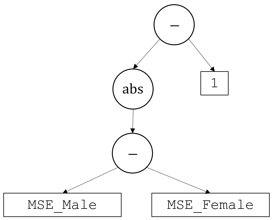
Consider an example where the user typed the following behavioral constraint: \(g(\theta)\)= |MSE_Male - MSE_Female| - 1. Here, MSE_Male and MSE_Female correspond to two base variables that we pre-specify and provide to the user—more generally, we could condition also on different state features, such as race, ethnicity, or other features. This would parse into the following tree:

Recall that the base variables MSE_Male and MSE_Female are ones that we have already built in by defining their corresponding unbiased estimators, \(\hat z\). Hence, just as we bounded \(g\) using \(\hat g\), we can bound \(z\) using \(\hat z\). This results in high-confidence bounds on both base variables. In this case we can automatically detect, by analyzing the parse tree, that we will need two-sided bounds (both upper and lower on these base variables). The image below depicts how the confidence intervals on the base variabes (and the constant 1, which can also be viewed as a base variable) are propagated through the tree to get a high-confidence upper bound on \(g(\theta)\).

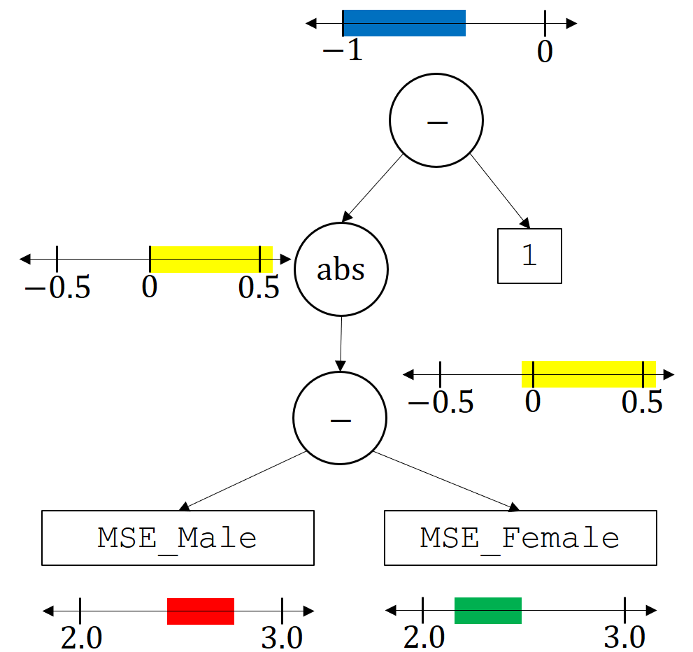
Here the red interval at the bottom is what we might obtain for the confidence interval on the base variable MSE_Male and the green interval is the confidence interval that we obtain for MSE_Female. When computing these, we require the confidence intervals on all base variables to hold simultaneously with probability \(\delta\). Consider the minus operator: we can obtain a high-confidence interval on the output of the minus operator by taking the maximum red value minus the minimum green value to obtain a high-confidence upper bound, and the smallest red value minus the biggest green value to obtain a high-confidence lower bound. These results are depicted in yellow on the right. The next operator, abs, makes any negative values positive, which in this case cuts off the negative values, as depicted in the yellow confidence interval on the left. Next, the top minus operator considers the confidence interval on the left minus one, giving the top blue confidence interval. As this is now a confidence interval on \(g(\theta)\), we check whether it is less than zero. Since it is, the solution \(\theta\) would pass the safety test and be returned. Notice that this process can be automated for arbitrary trees that correspond to the expressions entered by the user.

This interface can be further extended by allowing the user to provide unbiased estimators for other base variables that we didn't already think ahead to include, and by allowing the user to provide base variables for which they can compute confidence intervals given data, perhaps without constructing unbiased estimates (for an example, see Appendix G of our NeurIPS paper).

Reinforcement Learning

Extending QSA to the classification setting is straightforward. However, extending it to the reinforcement learning setting is slightly more challenging. In the regression and classification settings (both forms of supervised learning), we can easily estimate quantities like the mean squared error and false positive rates of a solution, \(\theta\), given data. We simply apply the solution to the data and compute the sample mean squared error or sample false positive rate. However, in the reinforcement learning setting we cannot "apply the solution to the data," since the choice of solution changes the distribution of data that would be generated.

In reinforcement learning, the problem of predicting what would happen if one solution (a policy) was used given data generated by a different solution (a different policy) is called off-policy evaluation or off-policy policy evaluation. The problem of obtaining confidence intervals around these predictions is called high-confidence off-policy policy evaluation (HCOPE). At the core of current Seldonian reinforcement learning algorithms are HCOPE algorithms that allow for high-confidence guarantees that the policy will only be changed when it is an improvement with respect to one or more reward functions (where reward functions could, for example, be labels on trajectories indicating whether an undesirable outcome occurred).

A complete review of HCOPE methods and reinforcement learning is beyond the scope of this tutorial. However, we refer the reader to the following sequence of papers, in order: 1, 2, 3, 4, 5, and 6. While there are many other fantastic papers in this area, these six provide a strong introduction.

Open Problems

The QSA algorithm that you have created, with the extention to reinforcement learning and the interface extentions listed above, is the current state-of-the-art in Seldonian algorithms. However, as you have seen, this algorithm is built from simple components and handles open problems with engineering hacks. This means that the field is wide open, waiting for your improved algorithms. Here we list some interesting open problems.

• How should the data be partitioned between the candidate and safety sets? Can this be phrased as an optimal stopping problem, where the candidate selection mechanism can pull as much data from the safety data set as it wants? If it pulls too little it will not produce a good candidate solution, while if it pulls too much the safety test's confidence intervals will be too loose to allow the candidate solution to pass.

• Doubling the width of the safety test's confidence interval, when predicting the safety test during candidate selection, is a hack. Can this be replaced with a more principled method for predicting the outcome of the safety test (perhaps with high confidence)?

• Is QSA consistent (under mild assumptions)? We have shown that a different Seldonian algorithm is consistent. This alternate algorithm is designed explicitly to facilitate this proof. Proving that QSA is consistent (under mild assumptions) would remove the need for the alternate design choices in that algorithm.

• How can we design even easier-to-use interfaces? Can the user communicate with natural language or by providing demonstrations?

• QSA does not tell the user why it returned NSF when it does. Can QSA return a reason as well, such as that it expects to require a certain amount more data to return a solution in the future, or that some of the constraints it was provided are conflicting or otherwise impossible to satisfy?

• Can we extend the Seldonian framework to sequential problems?

• If a Seldonian algorithm returns NSF, then the next time the algorithm is run it must use entirely new data in the safety test to avoid the problem of multiple comparisons. How can we modify QSA to allow us to intelligently re-use data (for example using confidence sequences or the reusable holdout)?

• Do other general algorithm designs work better in some cases? Other approaches could use multiple candidate policies (like the reinforcement learning algorithm in our Science paper) or algorithms that function entirely differently like SPI-BB and Fairlearn.

• There are many research areas within machine learning that might be extended to the Seldonian setting. Examples include differentially private algorithms, secure algorithms, multi-objective algorithms, continual learning algorithms, robust algorithms, and even deep learning algorithms.

• Can the search for the candidate solution be made particularly efficient in at least some cases?

• Can new and tighter high-confidence intervals be derived that enables algorithms to obtain the same performance with less data? For example, proving this inequality could provide drastic improvements in data-efficiency. Can confidence intervals on other quantities, like CVaR, variance, and entropy enable interesting new interfaces and behavioral constraints?

Hopefully you see the simplicity of the algorithms that we have presented so far, and ways in which they might be improved. Your improvements could enable Seldonian algorithms to operate using less data, or could provide users with improved interfaces. In either case, we hope that they will enable the responsible application of machine learning to future problems.