AI Safety · Tutorial 3

A Simple Seldonian Algorithm

Remember that we are following the three steps of the Seldonian framework:

Define the goal for the designer of the algorithm. Our goal is to create an algorithm $a$ that attempts to maximize an objective function $f$ and ensures that the behavioral constraints are satisfied. That is, we are searching for an algorithm $a$ that is an approximate solution to:

$$ \arg\max_{a \in \mathcal A}f(a)\\\text{s.t. }\forall i \in \{1,\dotsc,n\} \Pr(g_i(a(D)) \leq 0) \geq 1-\delta_i. $$

In this example, the goal is to create a regression algorithm $a$ that minimizes the negative MSE of the solution that $a$ returns for the user's application. Because we do not know the value of $f(a)$ for any $a$ (since we do not know, for instance, to which datasets the user will apply the algorithm), we allow the user to provide a sample objective function $\hat f:\Theta \times \mathcal D \to \mathbb R$ that acts as an estimate of the utility of any algorithm that returns the solution $\theta$, when given input data $D$. In our case, $\hat f(\theta,D)=\frac{1}{n}\sum_{i=1}^n (\hat y(X_i,\theta)-Y_i)^2$.

Define the interface that the user will use. We will begin by using an interface that makes creating the Seldonian algorithm easier. Our initial interface will require the user to provide functions $\hat g_i$, as described in the previous tutorial.

Create the algorithm.

We will implement the following algorithm.

First, the data $D$ is partitioned into two sets, $D_1$ and $D_2$. We call $D_1$ the candidate data and $D_2$ the safety data. Once the data has been partitioned, a method called Candidate Selection uses the candidate data to pick a single solution, $\theta_c$, called the candidate solution, which the algorithm considers returning. The candidate solution is then passed to the Safety Test mechanism, which uses the safety data to test whether the candidate solution is safe to return. If so, it is returned, and if not the algorithm returns No Solution Found (NSF).

A diagram of this algorithm is provided below.

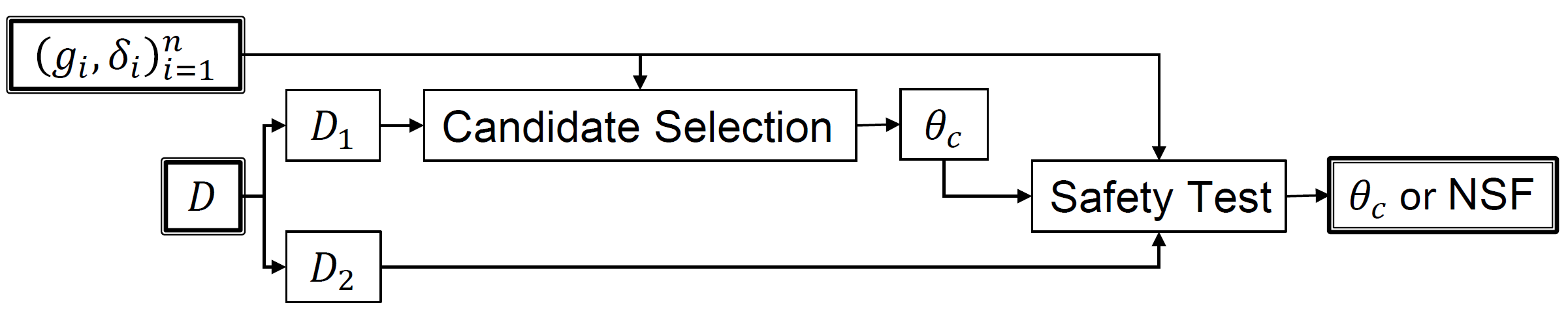
Figure S15 (supplemental materials) from P. S. Thomas, B. Castro da Silva, A. G. Barto, S. Giguere, Y. Brun, and E. Brunskill. Preventing undesirable behavior of intelligent machines. Science, 366:999–1004, 2019. Reprinted with permission from AAAS.

A common misconception is that this algorithm is the Seldonian algorithm. There is no such thing, just as there is no one algorithm that is the reinforcement learning algorithm. This is one example of a simple Seldonian algorithm and a simple interface.

The Safety Test Mechanism

Remember that a Seldonian algorithm ensures that, for all $i \in \{1,2,\dotsc,n\}$, $$\Pr(g_i(a(D))\leq 0)\geq 1-\delta_i.$$ The Safety Test mechanism is the component that ensures that these behavioral constraints hold. It does so using data, by computing a high-confidence upper bound on each $g_i(\theta)$ using a confidence interval derived from the Student $t$-statistic. If this high-confidence upper bound is less than or equal to zero for every behavioral constraint, then the candidate solution will be returned (we often say colloquially that the "solution is safe to return"); otherwise, the algorithm returns NSF.

The high-confidence upper bound on each $g_i(\theta)$ is computed as follows. Let $X=(X_1,\dotsc,X_m)$ be i.i.d. random variables. Under the assumption that $\frac{1}{m}\sum_{i=1}^m X_i$ is normally distributed, we can use the Student $t$-statistic to compute an upper bound on the expected value of these random variables: $$ \Pr\left (\mathbf E[X_1] \leq \hat \mu(X) + \frac{\hat \sigma(X)}{\sqrt{m}}t_{1-\delta,m-1} \right ) \geq 1-\delta, $$ where

$\hat \mu(v)$ and $\hat \sigma(v)$ are sample mean and sample standard deviation (with Bessel's correction) of a vector $v$. That is, $\hat \mu(v)=1/|v|\sum_{i=1}^{|v|}v_i$ and $\hat \sigma(v)=\sqrt{(|v|-1)^{-1}\sum_{i=1}^{|v|}(v_i-\hat \mu(v))^2}$, where $|v|$ is the number of elements in $v$; and
$t_{1-\delta,\nu}$ is the $100(1-\delta)$ percentile of the Student $t$-distribution with $\nu$ degrees of freedom, i.e., tinv($1-\delta,\nu$) in Matlab.

To construct the Safety Test mechanism, first remember that:

We will apply the safety test to a single solution, which we call the candidate solution, $\theta_c$.
$D_2$ is the data used by the Safety Test;
$\hat g_{i}(\theta_c)=(\hat g_{i,1}(\theta_c, D_2), \ldots, \hat g_{i,m}(\theta_c, D_2))$ is a vector containing $m$ i.i.d. values of $g_{i}(\theta_c)$; and
$\mathbf E[\hat g_{i,j}(\theta_c,D_2)]=g_i(\theta_c)$.

By substituting these into the high confidence upper bound discussed above, we have that $$ \Pr\left (g_i(\theta_c) \leq \hat \mu(\hat g_i(\theta_c,D_2)) + \frac{\hat \sigma(\hat g_i(\theta_c,D_2))}{\sqrt{|D_2|}}t_{1-\delta_i,|D_2|-1} \right) \geq 1-\delta_i. $$ This implies that, given a candidate solution $\theta_c$ and dataset $D_2$, $\left( \hat \mu(\hat g_i(\theta_c,D_2)) + \frac{\hat \sigma(\hat g_i(\theta_c,D_2))}{\sqrt{|D_2|}}t_{1-\delta_i,|D_2|-1} \right) $ is a high-confidence upper bound on $g_i(\theta_c)$. If this upper bound is less than or equal to zero, then $g_i(\theta_c)$ is less than or equal to zero with high probability. So, the Safety Test can satisfy the behavioral constraint by only returning $\theta_c$ when $\left( \hat \mu(\hat g_i(\theta_c,D_2)) + \frac{\hat \sigma(\hat g_i(\theta_c,D_2))}{\sqrt{|D_2|}}t_{1-\delta_i,|D_2|-1} \right) \leq 0$.

Notice that the upper bound above assumes that the vector of samples being analyzed, $\hat \mu(X)$, is normally distributed. This is reasonable if $m$ is sufficiently large, due to the central limit theorem.

Computing a Candidate Solution

With the safety test in place, the algorithm will be Seldonian regardless of how the candidate solution is computed, as long as it is not computed using the data $D_2$, which is used by the safety test. This is the reason why the algorithm splits the training data $D$ into two sets, $D_1$ (used to compute a candidate solution) and $D_2$ (used to perform the safety test).

First, consider what would happen if we computed a candidate solution $\theta_c$ as follows: $$\theta_c \in \arg\max_{\theta \in \Theta}\hat f(\theta,D_1).$$ In this case, the candidate solution would be one that performs well according to the primary objective, $\hat f$. However, this solution often will not be safe, and will fail the safety test, resulting in the algorithm returning NSF. To fix this, we want to select a candidate solution as follows: $$\theta_c \in \arg\max_{\theta \in \Theta}\hat f(\theta,D_1)\\\text{s.t. $\theta_c$ predicted to pass safety test}.$$ That is, we would like to only consider candidate solutions that we predict will pass the safety test. We can predict the result of the safety test by determining what it would return if it were to use the data set $D_1$ (the data set used to compute the candidate solution) instead of $D_2$: $$\theta_c \in \arg\max_{\theta \in \Theta}\hat f(\theta,D_1)\\\text{s.t. }\forall i \in \{1,2,\dotsc,n\},\quad \hat \mu(\hat g_i(\theta,D_1)) + \frac{\hat \sigma(\hat g_i(\theta,D_1))}{\sqrt{|D_2|}}t_{1-\delta_i,|D_2|-1}\leq 0.$$ Notice that the upper bound used above is identical to the one used in the Safety Test, except that the relevant statistics (mean $\hat \mu$ and standard deviation $\hat \sigma$) are computed over the dataset $D_1$, that is, the data set available to compute a candidate solution. Also notice that we are still using the size of the safety data set in two locations above.

The above method for computing the candidate solution can work well when the primary ojective and the behavioral constraints are aligned. However, when they are conflicting, the candidate selection mechanism tends to be over-confident that the candidate solution will pass the safety test (likely due to over-fitting on the candidate data). To fix this, we use a hack: we double the width of the confidence interval when predicting the outcome of the safety test, by multiplying the second term of the upper bound by two: $$\theta_c \in \arg\max_{\theta \in \Theta}\hat f(\theta,D_1)\\\text{s.t. }\forall i \in \{1,2,\dotsc,n\},\quad \hat \mu(\hat g_i(\theta,D_1)) + 2\frac{\hat \sigma(\hat g_i(\theta,D_1))}{\sqrt{|D_2|}}t_{1-\delta_i,|D_2|-1}\leq 0.$$

A Complete Algorithm

We can now present the complete algorithm by combining the two mechanisms introduced above:

Inputs: Feasible set $\Theta$, data $D$, probabilities $\delta_1,\delta_2,\dotsc,\delta_n$, functions $\hat g_1, \hat g_2, \dotsc, \hat g_n$, function $\hat f$.
Output: Either a solution in $\Theta$ or No Solution Found (NSF).
1. Partition $D$ into two data sets, $D_1$ and $D_2$.
2. Candidate Selection: Use a black-box optimization algorithm to compute $\theta_c$ that approximates a solution to: $$ \theta_c \in \arg\max_{\theta \in \Theta} \hat f(\theta,D_1)\\ \text{s.t. } \forall i \in \{1,2,\dotsc,n\}, \quad \hat \mu(\hat g_i(\theta,D_1)) + 2\frac{\hat \sigma(\hat g_i(\theta,D_1))}{\sqrt{|D_2|}}t_{1-\delta_i,|D_2|-1} \leq 0 $$
3. Safety Test: Return $\theta_c$ if $$ \forall i \in \{1,2,\dotsc,n\}, \quad \hat \mu(\hat g_i(\theta_c,D_2)) + \frac{\hat \sigma(\hat g_i(\theta_c,D_2))}{\sqrt{|D_2|}}t_{1-\delta_i,|D_2|-1} \leq 0, $$ and No Solution Found (NSF) otherwise.