AI Safety · Tutorial 2

Simple Problem: Hello Seldonian Machine Learning!

We begin with a simple problem that can be solved using a Seldonian algorithm. This is the Hello World! of Seldonian machine learning. When first solving this problem, we will hold off on providing a slick interface, and focus on the core computational components of a Seldonian algorithm.

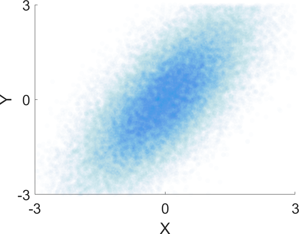
In this tutorial we will consider a regression problem. Let $X \in \mathbb R$ and $Y \in \mathbb R$ be two dependent random variables. Our goal is to estimate $Y$ given $X$, based on training data consisting of $m$ independent and identically distributed samples, $\{(X_i,Y_i)\}_{i=1}^m$. In this example we construct synthetic data where the inputs $X$ come from a standard normal distribution and where the outputs $Y$are equal to the inputs, plus noise with a standard normal distribution: $$ X \sim N(0,1)\quad\text{ and } \quad Y \sim N(X,1), $$ where $N(\mu,\sigma^2)$ denotes the normal distribution with mean $\mu$ and variance $\sigma^2$. Notice that Seldonian algorithms will not know the distributions of $X$ and $Y$ in advance.

The plot below shows 50,000 points sampled in this way:

Matlab source code: [link].

Let $\Theta = \mathbb R^2$ and let $\hat y(X,\theta)=\theta_1 X + \theta_2$ be the estimate of $Y$ given $X$ and $\theta$. The mean squared error (MSE) of a solution $\theta$ is $$ \operatorname{MSE}(\theta)=\mathbf E\left [ (\hat y(X,\theta)-Y)^2\right ]. $$ In our example, the goal of the designer of the algorithm is to construct an algorithm that

minimizes the mean squared error (or, equivalently, maximizes the negative of the MSE); and
ensures that, with probability at least 0.9, the mean squared error of its predictions is below 2.0; and that with probability at least 0.9, the mean squared error if its predictions is above 1.25.

In other words, the designer wishes to create an algorithm $a$ that maximizes $f(a)$ (where $f(a)$ is the negative MSE) and that satisfies $n=2$ behavioral constraints, $g_1$ and $g_2$, with probabilities $1-\delta_1$ and $1-\delta_2$, respectively. The behavioral constraints, then, are

$g_1(\theta)=\operatorname{MSE}(\theta)-2.0$ and $\delta_1=0.1$
$g_2(\theta)=1.25 - \operatorname{MSE}(\theta)$ and $\delta_2=0.1$

Because the algorithm does not have prior access to the distributions of $X$ and $Y$, it cannot compute $\operatorname{MSE}(\theta)$ analytically for any given candidate solution $\theta$. More generally, because we do not know the user's application—to which datasets he or she will apply the algorithm—we cannot compute the value of $f(a)$ for any $a$. We can, however, define a sample objective function, $\hat f$, that estimates the utility of a given algorithm, $a$, when $a$ returns the solution $\theta$ given input data $D$. In our particular example, the sample objective function $\hat f$ is the sample mean squared error of a given candidate solution $\theta$: $$ \hat f(\theta,D)=-\frac{1}{n}\sum_{i=1}^n (\hat y(X_i,\theta)-Y_i)^2. $$ Furthermore, notice that the behavioral constraints, $g_1$ and $g_2$, are also defined in terms of the MSE, which cannot be computed exactly. This means that $g_1$ and $g_2$ cannot be computed analytically either. Instead of requiring the user to produce $g_1$ and $g_2$, we allow the user to specify functions $\hat g_i$ that provide unbiased estimates of each corresponding constraint $g_i$. In particular, each function $\hat g_i(\theta,D)$ uses data to compute a vector of independent and identically distributed (i.i.d.) unbiased estimates of $g_i(\theta)$. Let $g_{i,j}(\theta,D)$ be the $j^\text{th}$ unbiased estimate returned by $\hat g_i(\theta,D)$. In our regression application, we compute these unbiased estimates of the behavioral constraints as follows:

$\hat g_{1,j}(\theta,D) = (\hat y(X_j,\theta)-Y_j)^2-2.0$, and
$\hat g_{2,j}(\theta,D) = 1.25-(\hat y(X_j,\theta)-Y_j)^2$.

Notice that because $g_{i,j}(\theta,D)$ are i.i.d. unbiased estimates of $g_i$, it follows that for every $i$ and $j$, $g_i(\theta)=\mathbf E[\hat g_{i,j}(\theta,D)]$.

Recap

A Seldonian algorithm $a$ maximizes an objective function $f$ and ensures that all behavioral constraints are satisfied.
In this example we wish to create a linear regression algorithm that guarantees with probabiliy $0.9$ that the MSE of its predictions is below $2.0$ and with probability $0.9$ that the MSE of its predictions is above $1.25$
By Boole's inequality, this implies that with probability $0.8$ the MSE of its predictions is in the interval $[1.25,2.0]$.
In our example, $f(a)$ is the negative MSE of the solution that algorithm $a$ will return for the user's application. We do not know the value of $f(a)$ for any $a$, as we do not know in advance the user's application when creating the algorithm.
Instead, we will require the user to provide a sample objective function, $\hat f:\Theta \times \mathcal D \to \mathbb R$, such that $\hat f(\theta,D)$ is an estimate of the utility of any algorithm that returns the solution $\theta$ when given input data $D$. In this example, $\hat f$ is the sample mean squared error: $\hat f(\theta,D)=\frac{1}{n}\sum_{i=1}^n (\hat y(X_i,\theta)-Y_i)^2$.
We will test our algorithm on a simple data set where the inputs come from a standard normal distribution and the outputs are equal to the inputs, plus noise with a standard normal distribution.
We will begin by using an interface that makes creating the Seldonian algorithm easier. Our initial interface will require the user to provide functions $\hat g_i$. Later we will focus on interfaces that make it easier for users to define and identify undesirable behavior.
Our example application was constructed to be simple, and yet also to test the ability of a Seldonian algorithm to handle behavioral constraints that may be in conflict with the objective function. Notice, for instance, that the solution that minimizes the MSE will violate the second behavioral constraint.
Once we have created a quasi-Seldonian algorithm for this problem, we will discuss how to create more powerful interfaces to specify undesirable behavior and how to apply these ideas to the general regression and classification settings.